Method

Categorical Methods

  • Method

Categorical analysis may best suit outcome variables with nominal or ordinal properties to describe associations applicable to healthy birth, growth, and development. Additionally, Ki can combine continuous outcome variables from collaborators by utilizing categories to align data, which may be differentially (continuous vs. categorical) collected across data sources.

UTILIZATION OF CATEGORICAL METHODS

Advantages of categorical methods

  • The parameters are easily interpretable (probabilities or odds of outcome).

Disadvantages of categorical methods

  • If continuous variables are categorized, a level of detail is lost.
  • Categories may lack clinical relevance, may include too few observations, or result in empty cells when many categories are created


WHAT ARE CATEGORICAL METHODS?

  • Regression models incorporate binary or multi-category outcome variables to determine risk or log odds of one category of an outcome compared to the reference category of the same outcome. Predictors can be either categorical or continuous.
  • Statistical methods that utilize categorical variables require different approaches, compared to continuous variables, due to the differences in statistical summaries and distributions.[1]
  • Categorical variables are best summarized using frequencies and percentages, which can be thought of as probabilities. The frequencies, by definition, must be greater than zero (non-negative numbers).
  • The natural logarithm is a commonly used transformation to ensure data is greater than zero (non-negative) and displays as a linear function of the predictor variable(s). However, this assumption can be relaxed by using flexible splines or other nonlinear functions.
  • The probabilities by definition must be between 0 and 1, and several transformation “link” functions can be used to map the probabilities from (0, 1) into an unconstrained scale (-∞, +∞). Common transformations include logit and probit.
  • Contingency tables, or two-by-two tables (a special case for two variables with two categories each), can provide a useful summary of categorical predictor and outcome variables. For example, Table 1 shows the stunting status at birth with the corresponding maternal Height category of the mother.

Ordinal Logistic Regression[3]

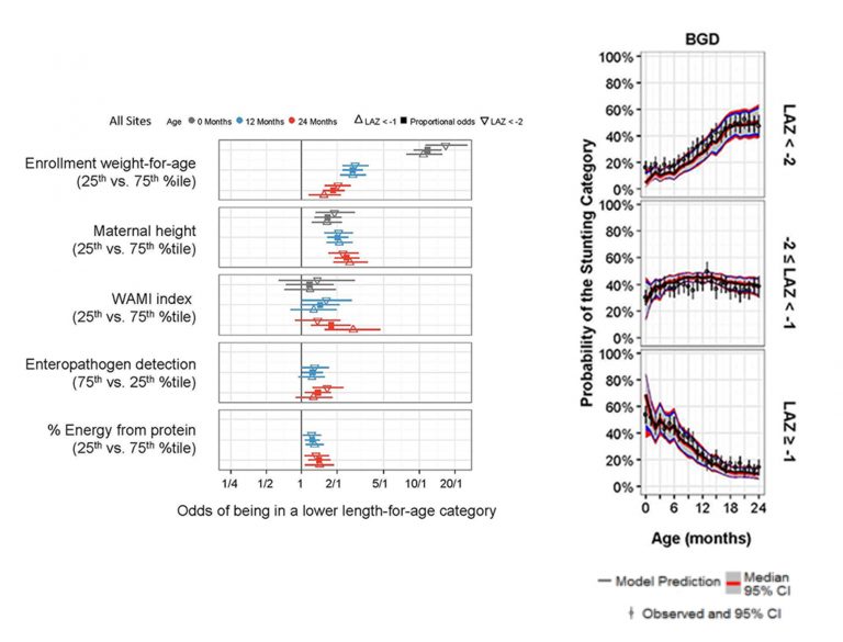
When trying to understand risk factors that are associated with ordered categorical outcomes, ordinal logistic regression (OLR) can be useful as described in the example that follows.  In the example, a set of independent variables (predictors) are selected to predict the odds of outcome being one of the ordered response categories (dependent variable).

This model assumes the proportionality of odds for each category of the response variable. In other words, the effect of the predictor is the same across the different categories, which means that for a given change of the predictor, the odds from passing from one category to the next is the same regardless of what category we are starting at. This test for proportionality is discussed further and displayed in the ki example below and can be relaxed if it does not hold.

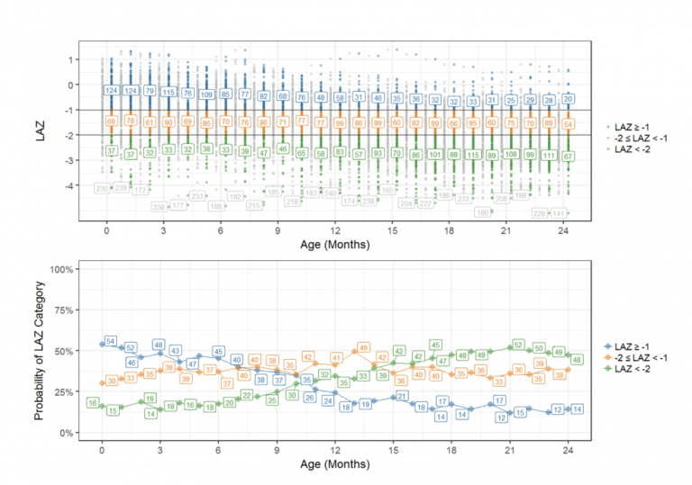
Example: Ordered categorical model for LAZ

As an example, an previous ki models have defineda categorical outcome variable for length-for-age-zscore (LAZ) where participants were defined as being stunted if LAZ < -2, at-risk for stunting if LAZ was between -2 and -1, and not stunted if LAZ ≥ -1.  LAZ was regressed on continuous and categorical variables including age, mother’s height, presence of enteric pathogens in stool, % energy from protein, enrollment LAZ and other important variables.[4] In Figure 1(upper panel), LAZ values have been color-coded to represent the 3 categories: stunted, at-risk for stunting, and not stunted.At age 0 Months, we had 37 infants below -2 (green points) from the total of 230 infants (shown in gray). This translates to the 16% shown age 0 Months in the lower panel of Figure 1. The probability of being stunted (LAZ < -2) is increasing over time (follow the green line).

To relate LAZ as an outcome of potential risk factors, ordinal regression analysis was utilized because of the natural order of the constructed LAZ categories .A linear piecewise spline age with breakpoints every 6-month intervals was necessary to describe the nonlinear relationship between age and the probability of LAZ category.

FIGURE 1. Categorization of LAZ outcome variable.[4]

FIGURE 2. Goodness of Fit example from MAL-ED study.[4] The median 95% CI helps visualize the fit of the model. FIGURE 3. Proportionality of odds assumption example from MAL-ED study.[4]

Figure 2 (on the right) illustrates the data over time and how to assess goodness of fit. The model for age (x-axis) as a predictor of the probability by LAZ category (y-axis) fits well (as shown by the overlap in the gray 95% confidence intervals and observed circular points with the model prediction[solid black line]).

Figure 3 (on the left) demonstrates that the proportionality of the odds assumption is met for 5 important risk factors for LAZ.  The overlap between the odds (solid square) and the two LAZ categories (triangles) indicates that proportionality did not meaningfully differ across LAZ categories, as demonstrated by the “substantial overlap” in the confidence intervals.

More Information on DISTRIBUTIONS[2]

Categorical data can be evaluated using statistical tests based on different distributional assumptions.

  • Binomial distribution is the probability distribution for the number of successful outcomes in a set of trials with two possible outcomes. This distribution approximates a normal distribution when the sample size is large.
  • Statistical inference uses maximum likelihood estimates, which are the parameters of a logistic regression, to identify which parameter values make the observed data most likely.

The parameter, or likelihood estimate, is dependent on the probability of the outcome.

  • The likelihood ratio test is a hypothesis test to evaluate the difference between the observed parameter and its null value which is usually zero (parameter has no impact on the probability). Another way of conceptualizing the likelihood ratio test is a test of whether the odds ratio confidence interval includes one, or there is no increased odds of the outcome in the presence of the predictor parameters. For example, we can have two logistic regression models of stunting, one with no predictors and one with maternal height (below median/above median) as a predictor. We then compare the two model’s likelihoods by comparing the ratio to a chi-square distribution with one degree of freedom (one parameter added in the model testing maternal height).
  • Chisquare (χ2) distribution is a probability density function that is right skewed. Its shape depends on the number of degrees of freedom (defined as n [observations] —1) and the total area under the curve (as any other probability distribution functions) equals one. Some of the statistical applications are:
    • Pearson’s Chi-squared testThis is a hypothesis test used to determine whether there is a statistical difference between the expected and observed frequencies in one or more categories. Example applications of this test include:
      • Independence Test: A hypothesis test to determine if an association is present between two observed proportions from a contingency table (Table 1).[1]
      • Homogeneity test: This is a hypothesis test to determine whether differences in distributions of variables vary between multiple populations.[1] For example, this test could be used to evaluate whether differences in the prevalence of stunting are present when comparing several different geographic regions.

TABLE 1. Example contingency table of stunting status at birth and maternal height category

References

  1. Weiss N. Introductory statistics. 9th ed. Boston: Pearson Addison- Wesley; 2012.
  2. Quigley D. Module 7.1: The Binomial, Chi-squared and Fisher’s Exact tests. 2016; http:// davidquigley.com/talks/2015/ biostatistics/module_07.1.html. Accessed Nov 2, 2017.
  3. Norusis M. IBM SPSS Statistics 19 Advanced Statistical Procedures Companion. Pearson; 2012.
  4. MAL-ED Network Investigators. Childhood stunting in relation to the pre- and postnatal environment during the first 2 years of life: The MAL-ED longitudinal birth cohort study. PLOS Medicine. 2017;14(10):e1002408.

Share

Last Updated

October, 2020